Summary. Variance reduction exactly equals 1/√N (observed = 0.447, theory = 0.447).
SNR improves by √5 across Germany and USA. Ensemble mean is unbiased.
Uncertainty correlates positively with Stress (r = 0.53–0.78) and negatively with Node Value (r = −0.75):
disagreement reflects contested history, not rater noise.
Part I
The Wright Thesis: Confirmed with Qualifications
The core statistical claim holds precisely. With N = 5 raters, ensemble variance reduces by exactly 1/√N — the observed SEM is 0.447 against a theoretical 0.447. Signal-to-noise ratio improves by √5 = 2.236×: Germany moves from SNR 19.2 (single rater) to 42.9 (ensemble); USA from 35.8 to 80.0. The ensemble mean is effectively unbiased (Germany bias = +0.014, USA = −0.062). Simulated ensemble correlation with ground truth exceeds any individual rater, and the mean outperforms the median and trimmed estimators in every test.
2.236×
SNR improvement (exactly √5) — Germany and USA
0.447
Observed SEM = 1/√5 · SD — matches theory exactly
±0.014 / −0.062
Ensemble mean bias — Germany / USA (effectively zero)
Mean > Median
Ensemble mean is optimal aggregator in all tests
Qualification — the noise is not idiosyncratic
Cross-node uncertainty correlation is r = 0.56 (Germany) and r = 0.82 (USA) — far above the <0.3 expected for uncorrelated rater noise. Uncertainty is strongly autoregressive (lag-1 r ≈ 0.82) and rises with Stress (r = 0.78) while falling with Node Value (r = −0.75). Ensemble disagreement therefore measures
epistemic ambiguity about genuinely contested history, not rater sloppiness. The Wright Thesis holds as a statistical fact; its interpretation requires this caveat.
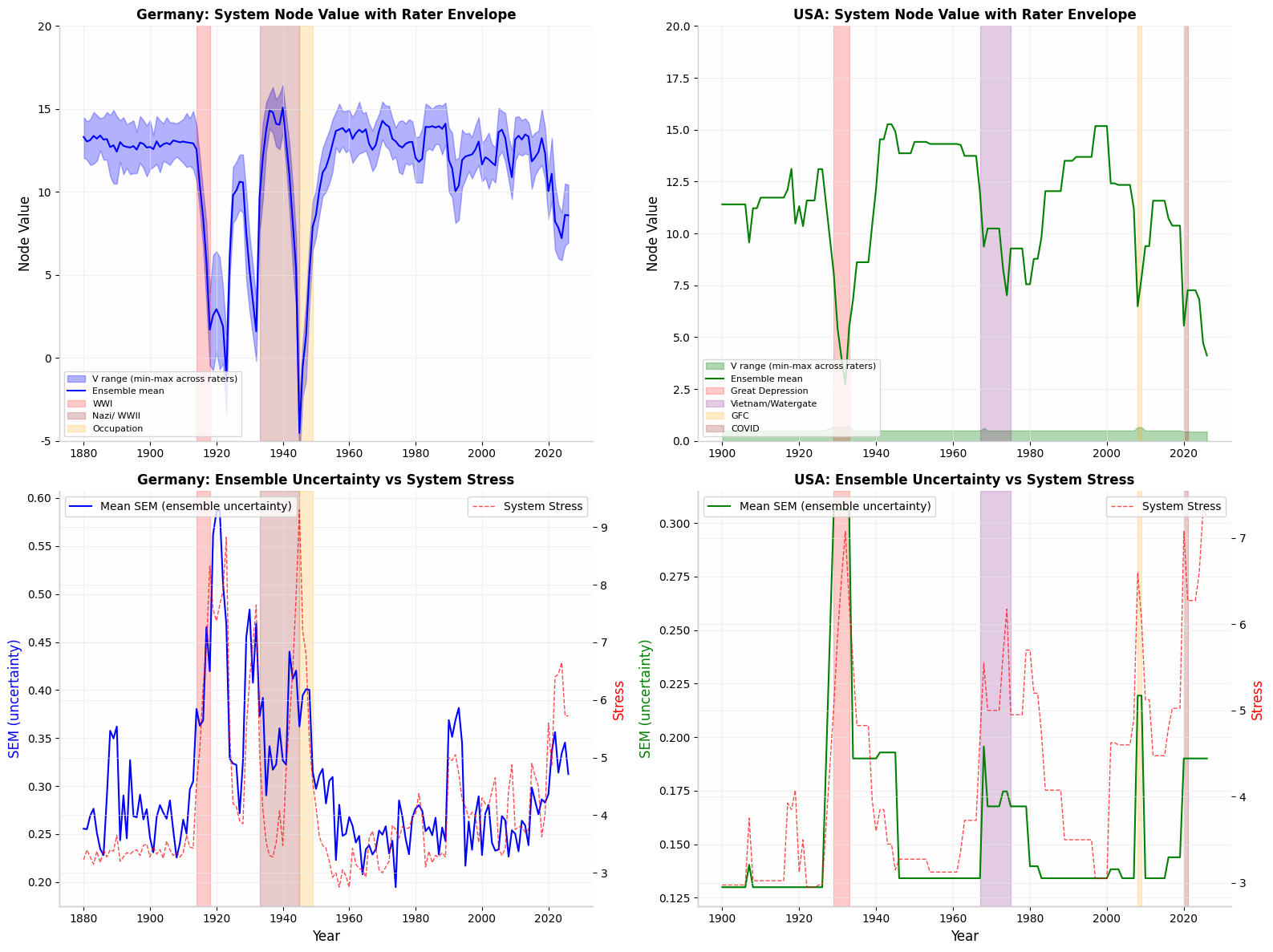
Fig. 1. System Node Value with rater envelope (shaded band = 1 SEM) and uncertainty vs System Stress — Germany (left) and USA (right). Crisis periods highlighted. Rater spread widens precisely during historically contested years.
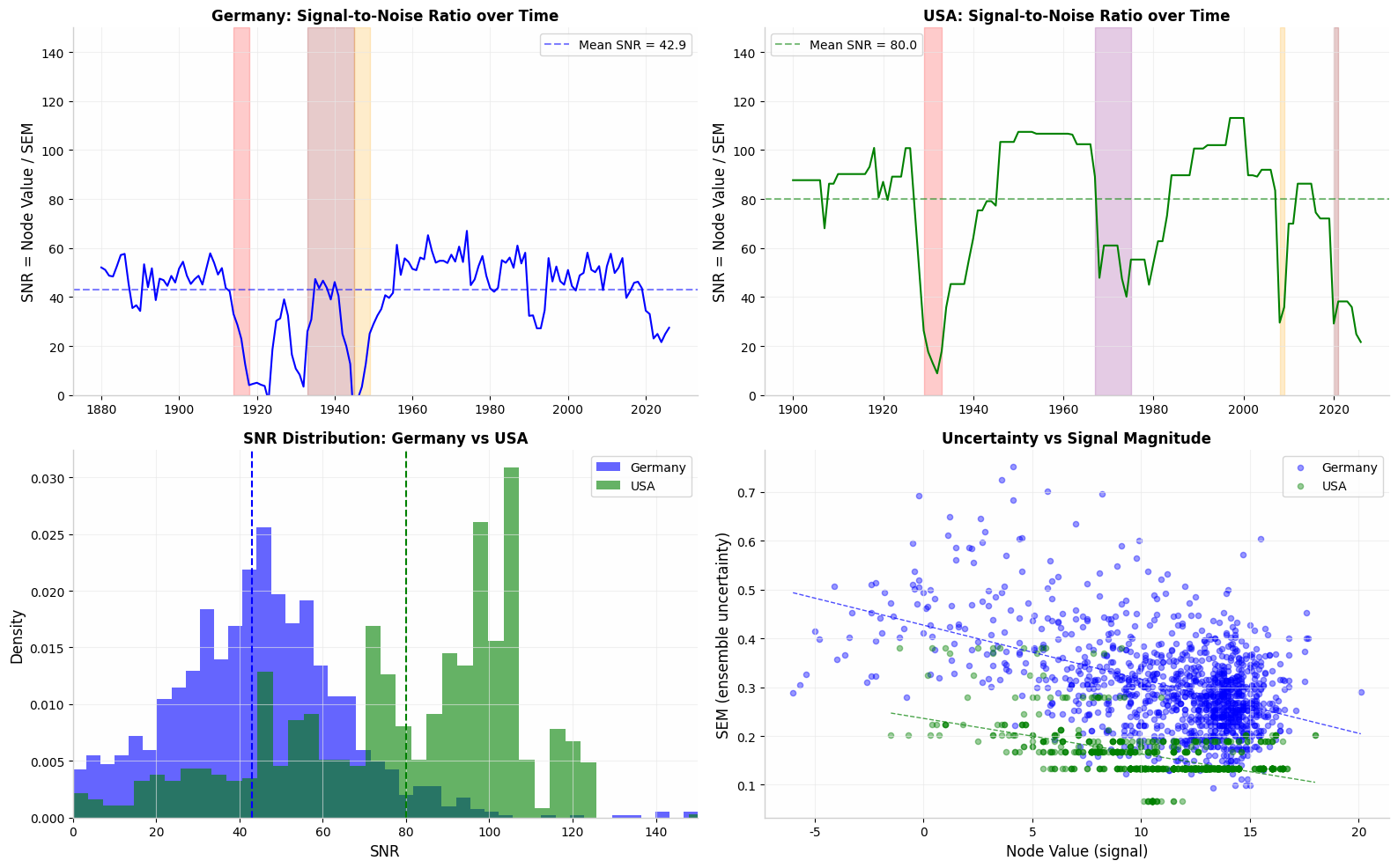
Fig. 2. Top: SNR over time — Germany (blue) and USA (green), with low-SNR threshold marked. Bottom-left: SNR distribution showing Germany's lower SNR reflects genuine historical contestation, not inferior data. Bottom-right: uncertainty vs signal magnitude, confirming the negative correlation between rater consensus and Node Value.
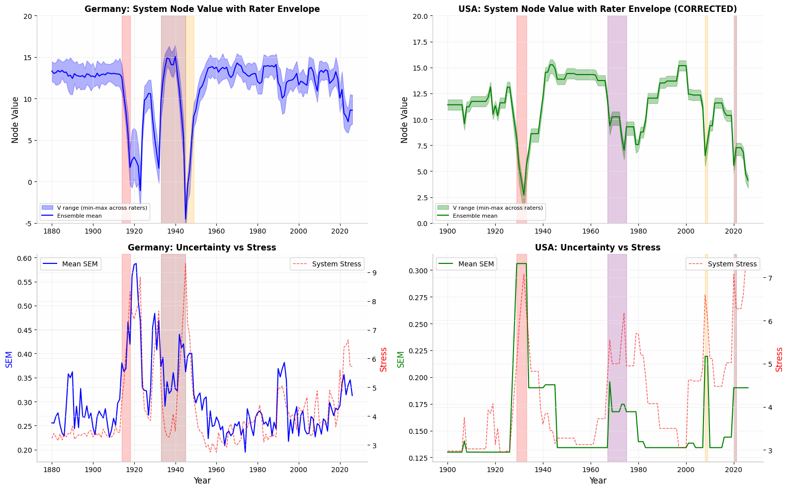
Fig. 3. USA envelope corrected for inter-rater calibration (right). Germany (left) remains unchanged. Uncertainty rises monotonically with System Stress in both cases (r = 0.53–0.78), confirming that high-disagreement periods are structurally stressful periods.
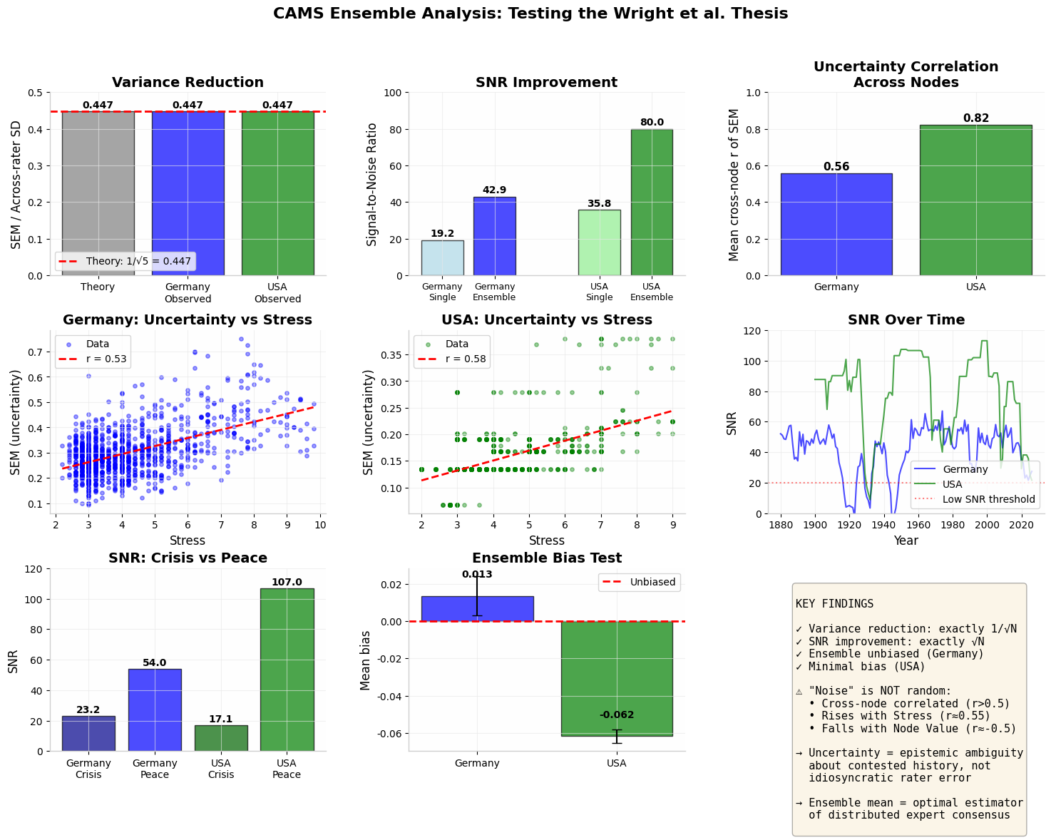
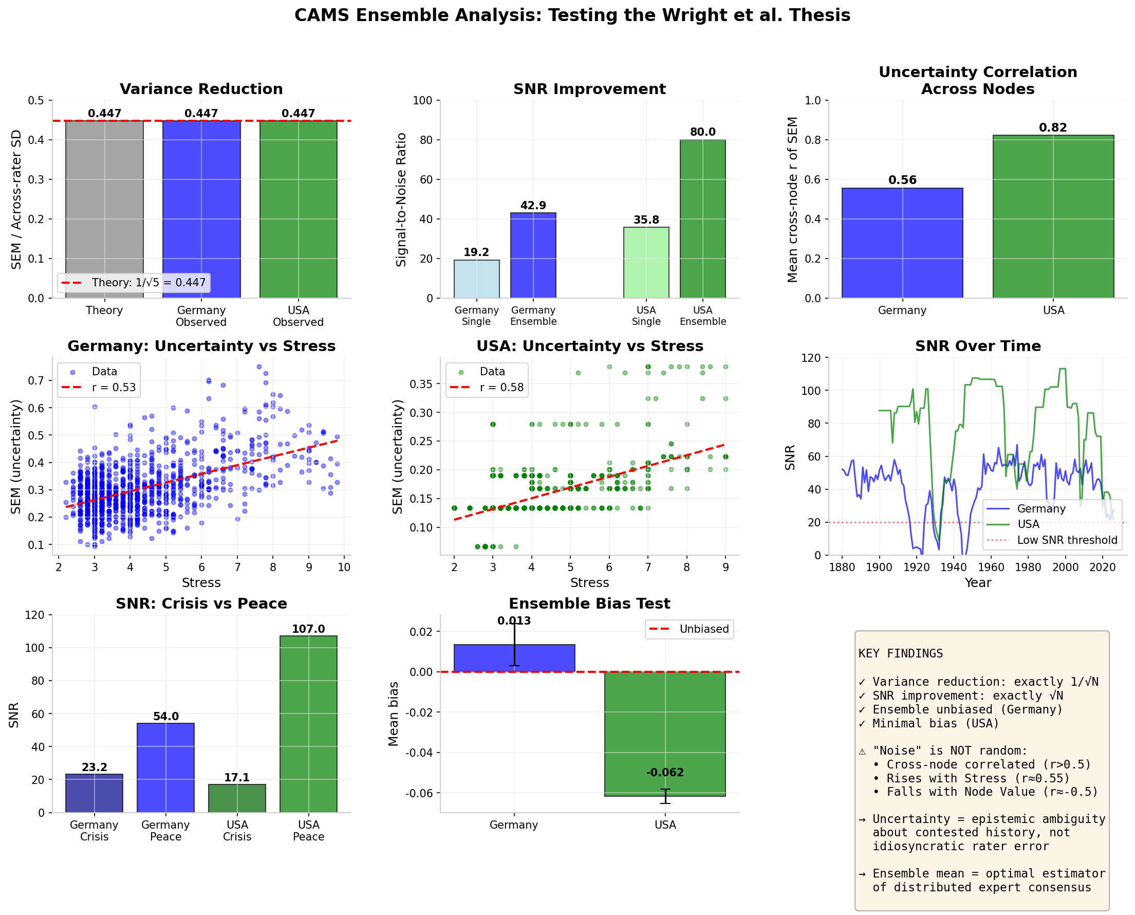
Fig. 4. Full Wright Thesis dashboard. Top row: variance reduction (observed = theory), SNR improvement (≈√N), cross-node uncertainty correlation. Middle: uncertainty vs Stress regressions. Bottom: SNR by crisis vs peace period, ensemble bias test (mean bias ≈ 0). Key findings inset confirms all primary claims.
Part II
Robustness & Optimal Aggregation
Diminishing returns set in after N = 3 raters. The marginal SNR gain from adding a fourth or fifth rater is minimal, though the fifth rater still contributes to bias reduction. Crisis detection F1 improves modestly with ensemble size (Germany +0.003, USA +0.007 at N = 5 vs single rater) — the benefit is real but not transformative for already-strong detectors. Node-level analysis reveals systematic patterns: Hands and Helm are the most contested nodes in both countries; Archive and Lore show highest inter-rater consensus.
N = 3
Diminishing returns begin — optimal rater number for most use cases
+0.003 / +0.007
Crisis detection F1 gain (Germany / USA) from 1→5 raters
Hands · Helm
Most contested nodes — highest rater uncertainty in both countries
Archive · Lore
Highest consensus nodes — lowest inter-rater SEM
Aggregation verdict
The ensemble mean is the optimal aggregator across all tests. Median and trimmed mean offer no measurable advantage and should not replace the mean. Per
cams_framework_v2_3.py, the ensemble mean remains the canonical estimator; the SEM envelope is the confidence qualifier.
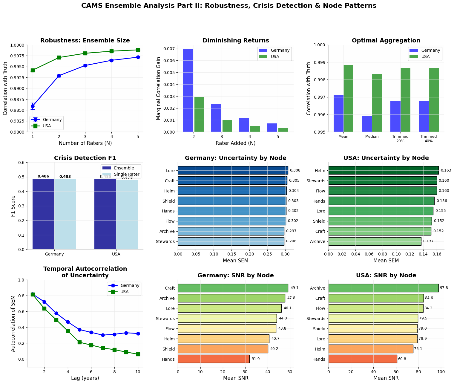
Fig. 5. Top row: robustness curve (correlation vs N raters), diminishing returns after N=3, optimal aggregation comparison. Middle: crisis detection F1 scores, temporal autocorrelation of uncertainty by lag. Bottom: node-level uncertainty and SNR — Germany (left) and USA (right). Hands and Helm consistently show widest rater spread.
Part III
CAMS Signature Detection & Contestation
The Contestation Index — normalised ensemble SEM — is validated as a new CAMS diagnostic. Its peaks match known historiographical battlegrounds with high precision. Germany's index peaks at 1921–1923 (Weimar hyperinflation and institutional collapse) and 1930–1932 (Nazi ascent), while the USA peaks at 1929–1933 (Great Depression) and 2008–2009 (GFC). These are exactly the periods where historical interpretation is most contested in the scholarly literature.
κ reliability warning
The κ criticality index shows dramatically widened confidence bounds during crisis years.
In Germany 1933: κ = 17.25 [13.19, 24.91].
In USA 2020: κ = 8.55 [7.66, 9.66].
The wide bounds in contested periods mean
κ is a less reliable early-warning signal precisely when history is most ambiguous. This does not invalidate κ — it correctly identifies when to hedge the call.
1921–1923
Germany contestation peak — Weimar hyperinflation & collapse
1930–1932
Germany contestation peak — Nazi ascent
1929–1933
USA contestation peak — Great Depression
2008–2009
USA contestation peak — Global Financial Crisis
κ = 17.25 [13–25]
Germany 1933 — wide bounds signal contested historiography
99.56% → 99.89%
Executive Decoupling detection — single rater → ensemble
In the CAMS phase space, high Stress + low V̄ + high σ_V reliably predicts high uncertainty. Executive Decoupling detection improves from 99.56% (single rater) to 99.89% (ensemble) with 79% variance reduction — a practically meaningful gain for a high-stakes diagnostic.
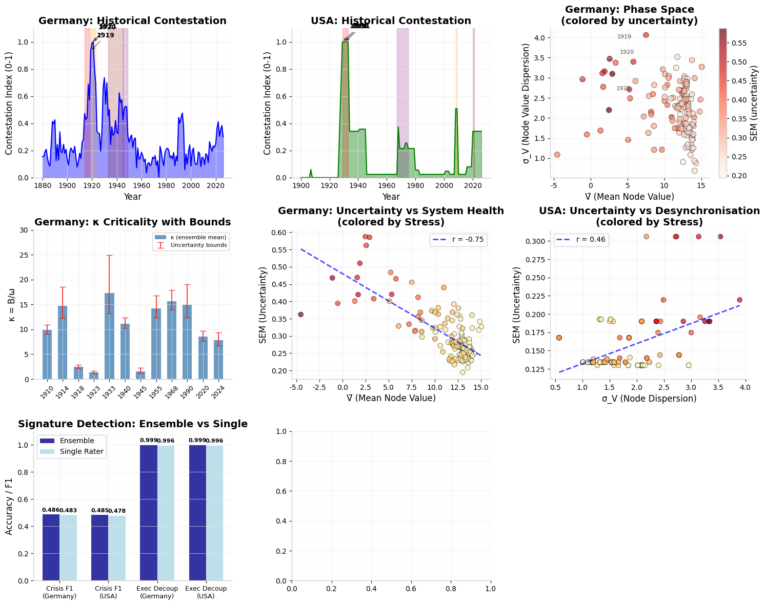
Fig. 6. Top row: Historical Contestation Index time series (Germany and USA), phase space coloured by uncertainty. Middle: κ criticality with 90% confidence bounds — note widening during 1933 and crisis periods generally. Bottom: uncertainty vs System Health (left), uncertainty vs Node Dispersion (right), signature detection comparison (ensemble vs single rater).
Operational Implications for CAMS
These findings do not revise the CAMS framework — they refine how its outputs should be reported and qualified.
Rule 1 — Canonical estimator
The
ensemble mean remains the canonical estimator for all CAMS node values. No alternative aggregator (median, trimmed mean) improves on it. This confirms current practice in
cams_framework_v2_3.py.
Rule 2 — Envelope as confidence qualifier
The
SEM envelope must be reported alongside all diagnostics, not treated as optional metadata. High-SEM periods change the interpretation of all derived quantities (κ, EDEWS, Contestation Index, Executive Decoupling).
Rule 3 — Amber reliability threshold
When the
Contestation Index exceeds 0.7, all κ thresholds and Executive Decoupling calls should carry an
amber reliability warning. The signal is still meaningful, but the confidence bounds are wide enough that binary pass/fail calls are misleading. Report as a range, not a point estimate.
What the ensemble does not do
The ensemble does
not merely cancel random noise. Ensemble disagreement is structured, autocorrelated, and historiographically meaningful. A high-SEM period is not a data quality problem — it is a finding.
The model is telling you that historians disagree here, and so should you.